Analysis of share market for mutual fund allocation & deriving relationship among different sector
Created by Achyut Ghosh and Soumik Bose
Contents
- Abstract
- Dimensions of Analysis
- Sample Dataset
- Different Regression Models
- Random Forest Regression
- Growth Rate Calculation
- Graphical Analysis
- Allocation of Funds
- Spreadsheet Example
- Finding The Relationship
- References
Abstract
- Share market prediction is always an interesting research topic as it deals with a lot of uncertainties and unpredictability.
- This project analyses the correlation between two different sectoral indices (e.g. between Automobile sector index and between Metal sector index, between Bank sector index and IT sectoral index etc.) in a time lagged manner.
Dimensions of Analysis
Time: Time is almost an inevitable dimension in data warehouse formation. For the share market Time could be represented in many formats: Hour, Day, Week, Month, Quarter, Year etc. as required for the analysis.
Dimensions of Analysis
Closing Price: “Closing price” generally refers to the last price at which a stock trades during a regular trading session. For Indian share market regular trading sessions run from 9:00 a.m. to 3:00 p.m.(GMT).
Dimensions of Analysis
Company Group: This could be represented in different ways, however, they are generally grouped to represent a specific industry (such as Banking, IT, Auto etc.) or based on market capitalization (such as Large Cap, Mid Cap, Small Cap).
Analyzing Dataset
- In this present work our main moto is to find the preferable method that would help us to predict the stock.
- Our prediction model is depend on technical analysis where all parameters are involved.
- Different regression models applied on scatter plot.
Sample Dataset
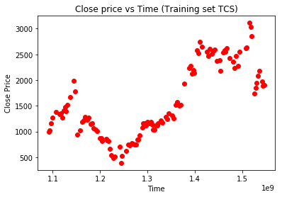
This is the scatter plot of sample dataset of TCS from Aug 2004 to Feb 2019.
Different Regression Models
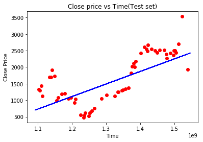
This is Linear Regression (TCS Month based) with R-squared value= 0.5234588
Different Regression Models
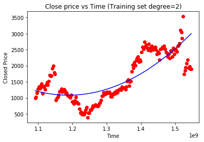
This is Polynomial Regression of degree 2 (TCS Month based) with R-squared value= 0.6379988
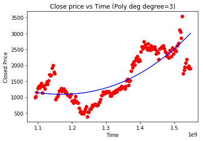
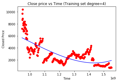
Different Regression Models

This is Polynomial Regression of degree 3 (TCS Month based) with R-squared value= 0.6126444
Random Forest Regression Model
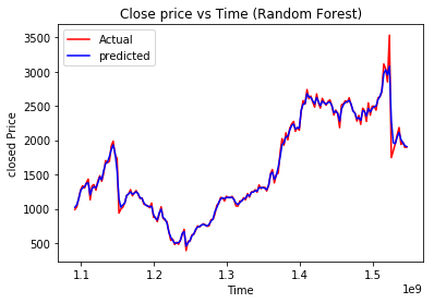
This is Randomforest Regression (TCS Month based) with R-Squared value=0.9909316
Random Forest Regression Psudo Code
						#Converting date into equivalent timeframe
						timestamp=[]
						import datetime
						import time
						for d in x:
						t=datetime.datetime.strptime(d[0],'%Y/%m/%d').date()
						ti=time.mktime(datetime.datetime
						.strptime(d[0], '%Y/%m/%d')
						.timetuple())
						timestamp.append([ti])

						#Fitting random forest regression for training set
						from sklearn.ensemble import RandomForestRegressor
						regressor =
						RandomForestRegressor(n_estimators = 80, random_state=0)
						regressor.fit(x_train,y_train)

						#Predicting the test set result
						y_pred=regressor.predict(x_test)
Growth Rate Calculation
- Pick up a company from a particular sector.
- Find the percentages of the growth rate of the company for a different time period with respect to the month immediate earlier.
Steps for calculation
- Deviation = Actual price-Predicted best fit price
- Weight = 1/(P *(p+1)/2), where P=Total Observation
- Growth = (Actual price of 2nd observation- Actual price of 1st observation)/ Actual price of 1st observation
- CNGR(Company Net Growth Rate) = Growth * Weight
- CNGRj = Y1 ∗ Gr1 + Y2 ∗ Gr2 + · · · + Yi ∗ Gri + · · · + Yp ∗ Grp, where CNGRj is the Company Net Growth Rate of jth company (where j=1 to m)
Growth Calculation Psudo Code
							#Deviation
							DeviationT=[]

							for i in range(0,174):
							Dev= Yt[i]-Y_pred_TCS[i]
							DeviationT.append(Dev)

							P_T=len(Yt)

							#compute Yi
							#formula 1
							m_Yi_T=[]
							Q=P_T
							#Weight Calculation
							Wt_T=1/(P_T * (P_T+1)/2)
							i=0
							while (i<244):
								Yi=Wt_T*Q
								m_Yi_T.append(Yi)
								i=i+1
							#compute Yi
							#formula 2
							for i in range(0,174):
							    Yi= Wt_T*Q
							    m_Yi_T.append(Yi)
								Q=Q-1

							######Step 3########
							Gr_T=[]
							G=0.0
							#for first growth is 0
							Gr_T.append(G)
							#Compute Growth(Gr)
							for i in range(1,174):
								 G=(Yt[i]-Yt[i-1])/Yt[i-1] * 100
								 Gr_T.append(G)
							#Company net growth Rate
							#CNGR
							CNGR_T=[]

							for i in range(0,174):
    						 	CN=Gr_T[i]*m_Yi_T[i]
    							CNGR_T.append(CN)
Graphical Analysis
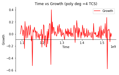
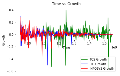
We have considered 3 IT Companies and Stock price started from January 2000 to Jan 2019
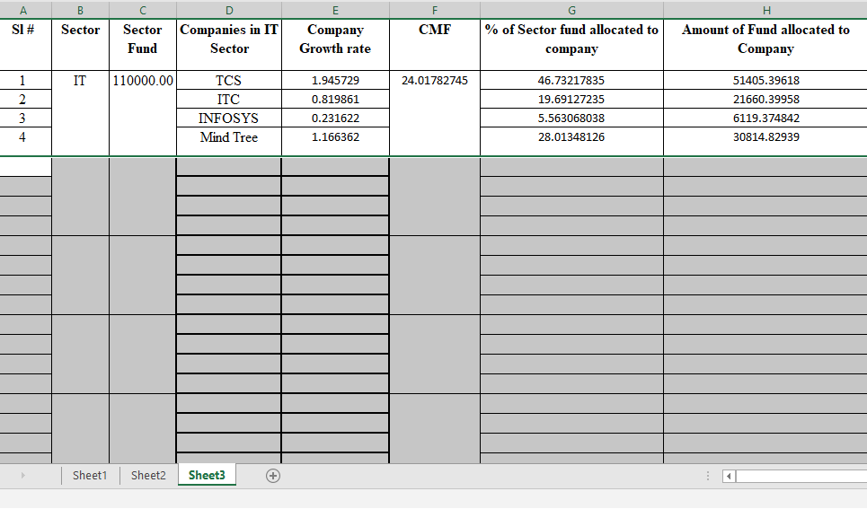
Allocation of Fund
- Our motive is to allocate more funds in such sectors and companies having better growth rate over the sectors.
- Find out the Company Multiplying Factor (CMF): CMF = 100/(Gr1 + Gr2 +…… Grn ), Where Gi is the growth rate of a company containing n number of companies.
Allocation of Fund
- Determine the company wise fund to be invested by the mathematical Formula given below.
CAk = gk × CMF for sector Ci, (where k = 1 to m ). Here CAk denotes company wise allocation percentage wise. - Thus company wise allocation is given by
SCAk = SFAi × CAk
Spreadsheet Example
Finding Relationship
- A correlation between different companies Growth indicates that if growth of certain Company increase or decrease what is the impact of that change into other Company's Growth.
- The Value of the Correlation varies from -1 to +1
Finding Relationship
Corelation coefficient of TCS & Infosys is -0.15566157 (Left) where as Corelation coefficient of TCS & ITC it is 0.08431221 (Right).
References
- Share Market Sectoral Indices Movement Forecast by Soumya Sen, Giridhar Maji & Amitrajit Sarkar
- Data
mining algorithm to analyse stock market
by Cicil Fonseka & Liwan H. Liyanage - Atsalakis GS, Valavanis KP (2009) Surveying stock market forecasting techniques - part ii: Soft computing methods. Expert Systems with Applications 36(3):5932 - 5941
References
- Basher SA, Sadorsky P (2006) Oil price risk and emerging stock markets. Global finance journal 17(2):224 - 251
- Chaudhuri S, Dayal U (1997) An overview of data warehousing and olap technology. ACM Sigmod record 26(1):65 - 74
- BSE Bombay Stock Exchange, India
- NSE National Stock Exchange, India.
- SEBI Securities & Exchange Board of India.
References
- Mingyue Q, Cheng L, Yu S (2016) Application of the artifical neural network in predicting the direction of stock market index. In: 2016 10th International Conference on Complex, Intelligent, and Software Intensive Systems (CISIS), IEEE, pp 219-223
- Mondal D, Maji G, Sen S, Goto T, Debnath NC (2017) A data warehouse based modelling technique for stock market analysis
- Sen S, Roy S, Sarkar A, Chaki N, Debnath NC (2014) Dynamic discovery of query path on the lattice of cuboids using hierarchical data granularity and storage hierarchy. Journal of Computational Science 5(4):675 - 683